Programming Bitcoin with Python
Learn how to generate private and public keys, and how to create a multi-signature bitcoin address in this tutorial with python.
In order to get started with bitcoin using Python, you must install Python 3.x and the bitcoin Python library called Pi Bitcoin tools in the system.
The Pi Bitcoin tools library
To install the Pi Bitcoin tools library, open the command-line program and execute the following command:
pip install bitcoin
The best thing about this library is that it does not need to have a bitcoin node on your computer in order for you to start using it. It connects to the bitcoin network and pulls data from places such as Blockchain.info.
For a start, write the equivalent of a Hello World program for bitcoin in Python. In the hello_bitcoin.py script, the demonstration of a new bitcoin address is created using Python. Go through the following steps to run the program:
1. Import the bitcoin library:
#!/usr/bin/env python

'''

Title - Hello Bitcoin

This program demonstrates the creation of

- private key,

- public key

- and a bitcoin address.

'''


# import bitcoin

from bitcoin import *
2. Generate a private key using the random key function:
my_private_key = random_key()
3. Display the private key on the screen:
print("Private Key: %s\n" % my_private_key)
How to generate private keys and public keys
With the private key, a public key is generated. Perform this step by passing the private key that was generated to the privtopub function, as shown here:
# Generate Public Key

my_public_key = privtopub(my_private_key)

print("Public Key: %s\n" % my_public_key)
Now, with the public key, generate a bitcoin address. Do this by passing the public key that is generated to the pubtoaddr function:
# Create a bitcoin address

my_bitcoin_address = pubtoaddr(my_public_key)

print("Bitcoin Address: %s\n" % my_bitcoin_address)
The following screenshot shows the private key, public key, and the bitcoin address that is generated:

Note that a bitcoin address is a single-use token. Just as people use email addresses to send and receive emails, you can use this bitcoin address to send and receive bitcoins. Unlike email addresses, however, people have several bitcoin addresses, and it is a must to use a unique address for every transaction.
Creating a multisignature bitcoin address
A multisignature address is an address that is associated with more than one private key. In this section, you’ll create three private keys. Multisignature addresses are useful in organizations where no single individual is trusted with authorising the spending of bitcoins.
Go through the following steps to create a multisignature bitcoin address:
- Create three private keys:
#!/usr/bin/env python

'''

Title - Create multi-signature address


This program demonstrates the creation of

Multi-signature bitcoin address.

'''

# import bitcoin

from bitcoin import *


# Create Private Keys

my_private_key1 = random_key()

my_private_key2 = random_key()

my_private_key3 = random_key()


print("Private Key1: %s" % my_private_key1)

print("Private Key2: %s" % my_private_key2)

print("Private Key3: %s" % my_private_key3)

print('\n')
2. Create three public keys from those private keys using the privtopub function:
# Create Public keys

my_public_key1 = privtopub(my_private_key1)

my_public_key2 = privtopub(my_private_key2)

my_public_key3 = privtopub(my_private_key3)


print("Public Key1: %s" % my_public_key1)

print("Public Key2: %s" % my_public_key2)

print("Public Key3: %s" % my_public_key3)

print('\n')
3. After generating the public keys, create the multisig by passing the three public keys to the mk_ multi-sig_script function. The resulting multisig is passed to the addr script function to create the multisignature bitcoin address.
# Create Multi-signature address

my_multi_sig = mk_multisig_script(my_private_key1, my_private_key2, my_private_key3, 2,3)

my_multi_address = scriptaddr(my_multi_sig)

print("Multi signature address: %s" % my_multi_address)
4. Print the multisignature address and execute the script. The following screenshot shows the output for the multisig bitcoin address:

You can also look at the preexisting bitcoin addresses’ transactional history. You’ll need to first get a valid address from Blockchain.info.
The following screenshot shows the copied address of a bitcoin block:

Pass the copied address to the history function, as shown in the following code, along with the output to get the history of the bitcoin address, including the transactional information:
!/usr/bin/env python

'''

Title - Bitcoin Transaction History


This program demonstrates listing history of a bitcoin address.

'''

# import bitcoin

from bitcoin import *


#View address transaction history

a_valid_bitcoin_address = '329e5RtfraHHNPKGDMXNxtuS4QjZTXqBDg'

print(history(a_valid_bitcoin_address))

Hope you found this article interesting. To learn more interesting stuff about bitcoins and Python, you can explore Hands-On Bitcoin Programming with Python. Written with an easy-to-understand approach in mind, Hands-On Bitcoin Programming with Python takes you through numerous practical examples to teach you to build software for mining and create bitcoin using Python.
Transforming Data in Different Ways in Pentaho
The set of operations covered in this tutorial is not a full list of the available options, but includes the most common ones, and will inspire you when you come to implement others.
Note that the files used in this tutorial were built with data downloaded from www.numbeo.com, a site containing information about living conditions in cities and countries worldwide. Before continuing, make sure you download the set of data from https://github.com/PacktPublishing/Pentaho-Data-Integration-Quick-Start-Guide.
Extracting data from existing fields
First, you’ll learn how to extract data from fields that exist in your dataset in order to generate new fields. For the first exercise, you’ll read a file containing data about the cost of living in Europe. The content of the file looks like this:
Rank City Cost of Living Index Rent Index Cost of Living Plus Rent Index Groceries Index Restaurant Price Index Local Purchasing Power Index

1 Zurich, Switzerland 141.25 66.14 105.03 149.86 135.76 142.70

2 Geneva, Switzerland 134.83 71.70 104.38 138.98 129.74 130.96

3 Basel, Switzerland 130.68 49.68 91.61 127.54 127.22 139.01

4 Bern, Switzerland 128.03 43.57 87.30 132.70 119.48 112.71

5 Lausanne, Switzerland 127.50 52.32 91.24 126.59 132.12 127.95

6 Reykjavik, Iceland 123.78 57.25 91.70 118.15 133.19 88.95

...
As you can see, the city field also contains the country name. The purpose of this exercise is to extract the country name from this field. In order to do this, go through the following steps:
- Create a new transformation and use a Text file input step to read the cost_of_living_europe.txt file.
- Drag a Split Fields step from the Transform category and create a hop from the Text file input towards the Split Fields step.
- Double-click the step and configure it, as shown in the following screenshot:

- Close the window and run a preview. You’ll see the following:


As you can see, the Split Fields step can be used to split the value of a field into two or more new fields. This step is perfect for the purpose of obtaining the country name because the values were easy to parse. You had a value, then a comma, then another value. This is not always the case, but PDI has other steps for doing similar tasks. Take a look at another method for extracting pieces from a field.
This time, you’ll read a file containing common daily food items and their prices. The file has two fields—food and price—and looks as follows:
Food Price

Milk (regular), (0.25 liter) 0.19 €

Loaf of Fresh White Bread (125.00 g) 0.24 €

Rice (white), (0.10 kg) 0.09 €

Eggs (regular) (2.40) 0.33 €

Local Cheese (0.10 kg) 0.89 €

Chicken Breasts (Boneless, Skinless), (0.15 kg) 0.86 €

...
Suppose that you want to split the Food field into three fields for the name, quantity, and number of units respectively. Taking the value in the first row, Milk (regular), (0.25 liter), as an example, the name would be Milk (regular), the quantity would be0.25, and the unit would be liter. You cannot solve this as you did before, but you can use regular expressions instead. In this case, the expression to use will be (.+)\(([0-9.]+)( liter| g| kg| head|)\).*.
Try it using the following steps:
- Create a new transformation and use a Text file input step to read the recommended_food.txt file. In order to define the Price as a number, use the format #.00 €.
- Drag a Regex Evaluation step from the Scripting category and create a hop from the Text file input toward this new step.
- Double-click the step and configure it as shown in the following screenshot. Don’t forget to check the Create fields for capture groups option:

- Close the window and run a preview. You will see the following:


The RegEx Evaluation step can be used just to evaluate whether a field matches a regular expression, or to generate new fields, as in this case. By capturing groups, you could create a new field for each group captured from the original field. You will also notice a field named result, which, in this example, has Y as its value. This Y means that the original field matched the given expression.
Note that while the Split Fields step removes the original field from the dataset, the RegEx Evaluation step does not.
These are not the only steps that will allow this kind of operation.
More ways to create new fields
Besides just extracting data from the incoming fields, you can also combine the fields by performing arithmetic operations between them, concatenating String fields, and using other methods. Just as in the previous section, this section will expand on a simple example that will serve you as a model for creating your own process.
For this tutorial, you’ll continue using the file containing data about the cost of living. This time, you’ll generate a new field that creates a new index out of the average of the restaurant price index and the groceries index. To do this, go through the following steps:
- Create a new transformation and use a Text file input step to read the cost_of_living_europe.txt file.
- Drag a Calculator step from the Transform category and create a hop from the Text file input toward the calculator.
- Double-click the step and configure it as shown in the following screenshot:

- Close the window and run a preview. You will see the following:


As you can deduce from the configuration window, with the Calculator step, you can create new fields by using temporary fields in the way. In the final dataset, you can see each temporary field—two and temp, in the example—as a new column.
The Calculator step is a handy step that can be used for performing many common types of operations, such as arithmetic, string, and date operations, among others.
Of course, there is a simpler way for doing the calculation in the last transformation:
- Save the previous transformation under a different name.
- Remove the Calculator step. You can do this just by selecting it and pressing Delete.
- Drag and drop a User Defined Java Expression step from the Scripting folder. Create a hop from the Text file input step toward this new step.
- Double-click the step and configure it as shown in the following screenshot:

- Close the window and run a preview. You should see exactly the same result as before.

The Java Expression step is a powerful step that allows you to create fields of any type—not just numbers—by using a wide variety of expressions, as long as they can be expressed in a single line using Java syntax.
In the last example, using the Java Expression step was simpler than doing the same with a Calculator step. Depending on the case, it can be more convenient to use one or the other.
This was just an example that showed you how to add new fields based on the fields in your dataset. There are many steps available, and with different purposes. You will find them mainly in the Transform folder, but there are some others in different folders in the Design tab. No matter which step you pick, the way you use it is always the same. You add the step at the end of the stream and then configure it properly according to your needs.
If you found this article interesting and helpful, you can check out Pentaho Data Integration Quick Start Guide. Featuring simplified and easy-to-follow examples, Pentaho Data Integration Quick Start Guide takes you through the underlying concepts in a lucid manner, so you can create efficient ETL processes using Pentaho.
Understanding React Pure Components
Many people are confused by the difference between a Functional Component and a Pure Component. Most of them think that they are the same, but this is not true. When you use a React Pure Component, We need to import PureComponent from React:
import React, { PureComponent } from 'react';
If your React component’s render method is “pure” (that means it renders the same result, given the same props and state), you can use this function to improve the performance of your application. A Pure Component performs a shallow comparison for the props and nextProps objects as well as the state and nextState objects. Pure components do not include the shouldComponentUpdate(nextProps, nextState) method, and if you try to add it, you’ll get a warning from React.
![]()
In this article, you’ll learn to create a basic example to understand how Pure Components works. To begin, you need to install the Chrome extension React Developer Tools to do a simple debug in your application. Download React Developer Tools from https://chrome.google.com/webstore/detail/react-developer-tools/fmkadmapgofadopljbjfkapdkoienihi.
Building your React application
First, create your React application using create-react-app. Once that is done, you can proceed to create your first React component.
Before you install create-react-app, remember that you need to download and install Node from www.nodejs.org. You can install it for Mac, Linux, and Windows.
Install create-react-app globally by typing this command in your Terminal:
npm install -g create-react-app
Alternatively, you can use a shortcut:
npm i -g create-react-app
Now build your first React application by following these steps:
- Create your React application with the following command:
create-react-app my-first-react-app
- Go to the new application with cd my-first-react-appand start it with npm start.
- The application should now be running at http://localhost:3000.
- Create a new file called js inside your src folder:
import React, { Component } from 'react';


class Home extends Component {

render() {

return <h1>I'm Home Component</h1>;

  }

}


export default Home;
File: src/Home.js
- You may have noticed that you are exporting your class component at the end of the file, but it’s fine to export it directly on the class declaration, like this:
import React, { Component } from 'react';

    export default class Home extends Component {

render() {

return<h1>I'm Home Component</h1>;

      }

    }
File: src/Home.js
- Now that you have created the first component, you need to render it. So, open the jsfile, import the Home component, and add it to the render method of the App component. If you are opening this file for the first time, you’ll probably see a code like this:
import React, { Component } from 'react';

import logo from './logo.svg';

import './App.css';

class App extends Component {

render() {

return (
 Welcome to React
);
}
}
export default App;
To get started, edit src/App.js and save to reload.
File: src/App.js
- Now change this code a bit. You need to import your Home component and then add it to the JSX. You also need to replace the <p> element with your component, like this:
import React, { Component } from 'react';

import logo from './logo.svg';


// We import our Home component here...

import Home from './Home';

import './App.css';

class App extends Component {

render() {

return (

Welcome to React
{/* Here we add our Home component to be render it */}

);} } export default App;
File: src/components/App.js
- Now, create the Numbers component:
// Dependencies

import React, { Component } from 'react';
// Components
import Result from './Result';

// Styles

import './Numbers.css';


class Numbers extends Component {

state = {

numbers: '', // Here we will save the input value

results: [] // In this state we will save the results of the sums

};

handleNumberChange = e => {

const { target: { value } } = e;


// Converting the string value to array

// "12345" => ["1", "2", "3", "4", "5"]

const numbers = Array.from(value);

// Summing all numbers from the array

 // ["1", "2", "3", "4", "5"] => 15

const result = numbers.reduce((a, b) => Number(a) + Number(b), 0);


// Updating the local state

this.setState({

numbers: value,

results: [...this.state.results, result]

});
}

render() {
return (
  {/* Rendering the results array */}
              {this.state.results.map((result, i) => (                               ))}

)       }     }   export default Numbers;
File: src/components/Numbers/Numbers.js
- Then, create the Result component (as a Class Component):
import React, { Component } from 'react';


class Result extends Component {

render() {

return<li>{this.props.result}</li>;

      }

    }


 export default Result;
File: src/components/Numbers/Result.js
- Finally, create the styles:
.Numbers {

      padding: 30px;

    }

.Numbers input[type=number]::-webkit-inner-spin-button,

    .Numbers input[type=number]::-webkit-outer-spin-button {

      -webkit-appearance: none;

      margin: 0;

    }


 .Numbers input {

      width: 500px;

      height: 60px;

      font-size: 20px;

      outline: none;

      border: 1px solid #ccc;

      padding: 10px;

    }


.Numbers ul {

      margin: 0 auto;

      padding: 0;

      list-style: none;

      width: 522px;

    }


 .Numbers ul li {

      border-top: 1px solid #ccc;

      border-left: 1px solid #ccc;

      border-right: 1px solid #ccc;

      padding: 10px;

    }


.Numbers ul li:first-child {

      border-top: none;

    }


.Numbers ul li:last-child {

      border-bottom: 1px solid #ccc;

    }
File: src/components/Numbers/Numbers.css
How React Pure Component works…
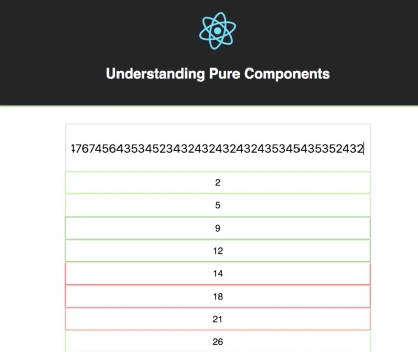
If you run the application, you will see this:

- You have used an input with the number type, which means you’ll only accept numbers if you start writing numbers (1, then 2, then 3, and such). You will see the results of the sum on each row (0 + 1 = 1, 1 + 2 = 3, 3 + 3 = 6):

Now, inspect the application using React Developer Tools. You need to enable the Highlight Updates option:

After this, start writing multiple numbers in the input (quickly), and you will see all the renders that React is performing:

As you can see, React is doing a lot of renderings. When the highlights are red, it means the performance of that component is not good. Here’s when React Pure Components will help you. Migrate your Result component to be a Pure Component:
import React, { PureComponent } from 'react';


class Result extendsPureComponent {

render() {

return <li>{this.props.result}</li>;

      }

    }


   export default Result;
File: src/components/Numbers/Result.js
Now if you try to do the same with the numbers, see the difference:

With the Pure Component React, you do less renders in comparison to a Class Component. Probably, you may now think that if you use a Stateless component instead of a Pure Component, the result will be the same. Unfortunately, this won’t happen. If you want to verify this, change the Result component again and convert it into a Functional Component.:
import React from 'react';


const Result = props => <li>{props.result}</li>;


 export default Result;
File: src/components/Numbers/Result.js
See what happens with the renders:
As you can see, the result is the same as the Class Component. This means that using a Stateless Component will not help you improve the performance of your application all the time. If you have components that you consider are pure, consider converting them into Pure components.
If you found this article interesting, you can explore Carlos Santana Roldan’s React Cookbook to be on the road to becoming a React expert. React Cookbook has over 66 hands-on recipes that cover UI development, animations, component architecture, routing, databases, testing, and debugging with React.
How to Use the jcmd Command for the JVM
This article will focus on the diagnostic command introduced with Java 9 as a command-line utility, jcmd. If the bin folder is on the path, you can invoke it by typing jcmd on the command line. Otherwise, you have to go to the bin directory or prepend the jcmd in your examples with the full or relative (to the location of your command line window) path to the bin folder.
If you open the bin folder of the Java installation, you can find quite a few command-line utilities there. These can be used to diagnose issues and monitor an application deployed with the Java Runtime Environment (JRE). They use different mechanisms to get the data they report. The mechanisms are specific to the Virtual Machine (VM) implementation, operating systems, and release. Typically, only a subset of these tools is applicable to a given issue.
If you do type it and there is no Java process currently running on the machine, you’ll get back only one line, as follows:
87863 jdk.jcmd/sun.tools.jcmd.JCmd
This shows that only one Java process is currently running (the jcmd utility itself) and it has the process identifier(PID) of 87863 (which will be different with each run).
JAVA Example
Now run a Java program, for example:
java -cp ./cookbook-1.0.jar

                   com.packt.cookbook.ch11_memory.Chapter11Memory
The output of jcmd will show (with different PIDs) the following:
87864 jdk.jcmd/sun.tools.jcmd.JCmd

87785 com.packt.cookbook.ch11_memory.Chapter11Memory
If entered without any options, the jcmd utility reports the PIDs of all the currently running Java processes. After getting the PID, you can then use jcmd to request data from the JVM that runs the process:
jcmd 88749 VM.version
Alternatively, you can avoid using PID (and calling jcmd without parameters) by referring to the process by the main class of the application:
jcmd Chapter11Memory VM.version
You can read the JVM documentation for more details about the jcmd utility and how to use it.
How to do it…
jcmd is a utility that allows you to issue commands to a specified Java process:
- Get the full list of the jcmdcommands available for a particular Java process by executing the following line:
jcmd PID/main-class-name help
Instead of PID/main-class, enter the process identifier or the main class name. The list is specific to JVM, so each listed command requests the data from the specific process.
- In JDK 8, the following jcmdcommands were available:
JFR.stop

JFR.start

JFR.dump

JFR.check

VM.native_memory

VM.check_commercial_features

VM.unlock_commercial_features

ManagementAgent.stop

ManagementAgent.start_local

ManagementAgent.start

GC.rotate_log

Thread.print

GC.class_stats

GC.class_histogram

GC.heap_dump

GC.run_finalization

GC.run

VM.uptime

VM.flags

VM.system_properties

VM.command_line

VM.version
JDK 9 introduced the following jcmd commands (JDK 18.3 and JDK 18.9 did not add any new commands):
- queue: Prints the methods queued for compilation with either C1 or C2 (separate queues)
- codelist: Prints n-methods (compiled) with full signature, address range, and state (alive, non-entrant, and zombie), and allows the selection of printing to stdout, a file, XML, or text printout
- codecache: Prints the content of the code cache, where the JIT compiler stores the generated native code to improve performance
- directives_add file: Adds compiler directives from a file to the top of the directives stack
- directives_clear: Clears the compiler directives stack (leaves the default directives only)
- directives_print: Prints all the directives on the compiler directives stack from top to bottom
- directives_remove: Removes the top directive from the compiler directives stack
- heap_info: Prints the current heap parameters and status
- finalizer_info: Shows the status of the finalizer thread, which collects objects with a finalizer (that is, a finalize()method)
- configure: Allows configuring the Java Flight Recorder
- data_dump: Prints the Java Virtual Machine Tool Interface data dump
- agent_load: Loads (attaches) the Java Virtual Machine Tool Interface agent
- status: Prints the status of the remote JMX agent
- print: Prints all the threads with stack traces
- log [option]: Allows setting the JVM log configuration at runtime, after the JVM has started (the availability can be seen using VM.log list)
- info: Prints the unified JVM info (version and configuration), a list of all threads and their state (without thread dump and heap dump), heap summary, JVM internal events (GC, JIT, safepoint, and so on), memory map with loaded native libraries, VM arguments and environment variables, and details of the operation system and hardware
- dynlibs: Prints information about dynamic libraries
- set_flag: Allows setting the JVM writable(also called manageable) flags
- stringtableand VM.symboltable: Print all UTF-8 string constants
- class_hierarchy [full-class-name]: Prints all the loaded classes or just a specified class hierarchy
- classloader_stats: Prints information about the classloader
- print_touched_methods: Prints all the methods that have been touched (have been read at least) at runtime
As you can see, these new commands belong to several groups, denoted by the prefix compiler, garbage collector (GC), Java Flight Recorder (JFR), Java Virtual Machine Tool Interface (JVMTI), Management Agent (related to remote JMX agent), thread, and VM.
How it works…
- To get help for the jcmdutility, run the following command:
jcmd -h
Here is the result of the command:

It tells you that the commands can also be read from the file specified after -f, and there is a PerfCounter.print command, which prints all the performance counters (statistics) of the process.
- Run the following command:
jcmd Chapter11Memory GC.heap_info
The output may look similar to this screenshot:

It shows the total heap size and how much of it was used, the size of a region in the young generation and how many regions are allocated, and the parameters of Metaspace and class space.
- The following command is very helpful in case you are looking for runaway threads or would like to know what else is going on behind the scenes:
jcmd Chapter11Memory Thread.print
Here is a fragment of the possible output:

- This command is probably used most often, as it produces a wealth of information about the hardware, the JVM process as a whole, and the current state of its components:
jcmd Chapter11Memory VM.info
It starts with a summary, as follows:

The general process description is as follows:
Then the details of the heap are shown (this is only a tiny fragment of it):

It then prints the compilation events, GC heap history, de-optimization events, internal exceptions, events, dynamic libraries, logging options, environment variables, VM arguments, and many parameters of the system running the process.
The jcmd commands give a deep insight into the JVM process, which helps to debug and tune the process for best performance and optimal resource usage.
If you found this article interesting, you can dive into Java 11 Cookbook – Second Edition to explore the new features added to Java 11 that will make your application modular, secure, and fast. Java 11 Cookbook – Second Edition offers a range of software development solutions with simple and straightforward Java 11 code examples to help you build a modern software system.
How to Develop a Real-Time Object Detection Project
Developing a real-time object detection project
You can develop a video object classification application using pre-trained YOLO models (that is, transfer learning), Deeplearning4j (DL4J), and OpenCV that can detect labels such as cars and trees inside a video frame. You can find the relevant code files for this tutorial at https://github.com/PacktPublishing/Java-Deep-Learning-Projects/tree/master/Chapter06. This application is also about extending an image detection problem to video detection. Time to get started!
Step 1 – Loading a pre-trained YOLO model
Since Alpha release 1.0.0, DL4J provides a Tiny YOLO model via ZOO. For this, you need to add a dependency to your Maven friendly pom.xml file:
<dependency>

  <groupId>org.deeplearning4j</groupId>

  <artifactId>deeplearning4j-zoo</artifactId>

  <version>${dl4j.version}</version>

</dependency>
Apart from this, if possible, make sure that you utilize the CUDA and cuDNN by adding the following dependencies:
<dependency>

  <groupId>org.nd4j</groupId>

  <artifactId>nd4j-cuda-9.0-platform</artifactId>

  <version>${nd4j.version}</version>

</dependency>

<dependency>

  <groupId>org.deeplearning4j</groupId>

  <artifactId>deeplearning4j-cuda-9.0</artifactId>

  <version>${dl4j.version}</version>

</dependency>
Now, use the below code to load the pre-trained Tiny YOLO model as a Computation Graph. You can use the PASCAL Visual Object Classes (PASCAL VOC) dataset (see more at http://host.robots.ox.ac.uk/pascal/VOC/) to train the YOLO model.
private ComputationGraph model;

private TinyYoloModel() {

        try {

            model = (ComputationGraph) new TinyYOLO().initPretrained();

            createObjectLabels();

        } catch (IOException e) {

            throw new RuntimeException(e);

        }

    }
In the above code segment, the createObjectLabels() method refers to the labels from the PASCAL Visual Object Classes (PASCAL VOC) dataset. The signature of the method can be seen as follows:
private HashMap<Integer, String> labels;

void createObjectLabels() {

        if (labels == null) {

            String label = "aeroplanen" + "bicyclen" + "birdn" + "boatn" + "bottlen" + "busn" + "carn" +

                    "catn" + "chairn" + "cown" + "diningtablen" + "dogn" + "horsen" + "motorbiken" +

                    "personn" + "pottedplantn" + "sheepn" + "sofan" + "trainn" + "tvmonitor";

            String[] split = label.split("\n");

            int i = 0;

            labels = new HashMap<>();

            for(String label1 : split) {

                labels.put(i++, label1);

            }

        }

    }
Now, create a Tiny YOLO model instance:
static final TinyYoloModel yolo = new TinyYoloModel();

    public static TinyYoloModel getPretrainedModel() {

        return yolo;

    }
Take a look at the model architecture and the number of hyper parameters in each layer:
TinyYoloModel model = TinyYoloModel.getPretrainedModel(); System.out.println(TinyYoloModel.getSummary());

Your Tiny YOLO model has around 1.6 million parameters across its 29-layer network. However, the original YOLO 2 model has more layers. You can look at the original YOLO 2 at https://github.com/yhcc/yolo2/blob/master/model_data/model.png.
Step 2 – Generating frames from video clips
To deal with real-time video, you can use video processing tools or frameworks such as JavaCV that can split a video into individual frames. Take the image height and width. For this, include the following dependency in the pom.xml file:
<dependency>

  <groupId>org.bytedeco</groupId>

  <artifactId>javacv-platform</artifactId>

  <version>1.4.1</version>

</dependency>
JavaCV uses wrappers from the JavaCPP presets of libraries commonly used by researchers in the field of computer vision (for example, OpenCV and FFmpeg). It provides utility classes to make their functionality easier to use on the Java platform, including Android.
For this project, there are two video clips (each 1 minute long) that should give you a glimpse into an autonomous driving car. This dataset has been downloaded from the following YouTube links:
- Building Self Driving Car – Local Dataset – Day: https://www.youtube.com/watch?v=7BjNbkONCFw
- Building Self Driving Car – Local Dataset – Night: https://www.youtube.com/watch?v=ev5nddpQQ9I
After downloading them, they were renamed as follows:
- SelfDrivingCar_Night.mp4
- SelfDrivingCar_Day.mp4
When you play these clips, you’ll see how Germans drive their cars at 160 km/h or even faster. Now, parse the video (first use day 1) and see some properties to get an idea of video quality hardware requirements:
String videoPath = "data/SelfDrivingCar_Day.mp4";

FFmpegFrameGrabber frameGrabber = new FFmpegFrameGrabber(videoPath);

frameGrabber.start();

Frame frame;

double frameRate = frameGrabber.getFrameRate();

System.out.println("The inputted video clip has " + frameGrabber.getLengthInFrames() + " frames");

System.out.println("Frame rate " + framerate + "fps");
>>>
 The inputted video clip has 1802 frames. The inputted video clip has frame rate of 29.97002997002997.
The inputted video clip has 1802 frames. The inputted video clip has frame rate of 29.97002997002997.
Now grab each frame and use Java2DFrameConverter to convert frames to JPEG images:
Java2DFrameConverter converter = new Java2DFrameConverter();

// grab the first frame

frameGrabber.setFrameNumber(1);

frame = frameGrabber.grab();

BufferedImage bufferedImage = converter.convert(frame);

System.out.println("First Frame" + ", Width: " + bufferedImage.getWidth() + ", Height: " + bufferedImage.getHeight());


// grab the second frame

frameGrabber.setFrameNumber(2);

frame = frameGrabber.grab();

bufferedImage = converter.convert(frame);

System.out.println("Second Frame" + ", Width: " + bufferedImage.getWidth() + ", Height: " + bufferedImage.getHeight());
>>>

  First Frame: Width-640, Height-360 Second Frame: Width-640, Height-360
The above code will generate 1,802 JPEG images against an equal number of frames. Take a look at the generated images:

Thus, the 1-minute long video clip has a fair number (that is, 1,800) of frames and is 30 frames per second. In short, this video clip has 720p video quality. So, you can understand that processing this video should require good hardware; in particular, having a GPU configured should help.
Step 3 – Feeding generated frames into the Tiny YOLO model
Now that you know some properties of the clip, start generating the frames to be passed to the Tiny YOLO pre-trained model. First, look at a less important but transparent approach:
private volatileMat[] v = new Mat[1];

private String windowName = "Object Detection from Video";

try {

    for(int i = 1; i < frameGrabber.getLengthInFrames();

    i+ = (int)frameRate) {

                frameGrabber.setFrameNumber(i);

                frame = frameGrabber.grab();

                v[0] = new OpenCVFrameConverter.ToMat().convert(frame);

                model.markObjectWithBoundingBox(v[0], frame.imageWidth,

                                               frame.imageHeight, true, windowName);

                imshow(windowName, v[0]);


                char key = (char) waitKey(20);

                // Exit on escape:

                if (key == 27) {

                    destroyAllWindows();

                    break;

                }

            }

        } catch (IOException e) {

            e.printStackTrace();

        } finally {

            frameGrabber.stop();

        }

        frameGrabber.close();
In the above code, you send each frame to the model. Then, you use the Mat class to represent each frame in an n-dimensional, dense, numerical multi-channel (that is, RGB) array.
In other words, you split the video clip into multiple frames and pass into the Tiny YOLO model to process them one by one. This way, you applied a single neural network to the full image.
Step 4 – Real Object detection from image frames
Tiny YOLO extracts the features from each frame as an n-dimensional, dense, numerical multi-channel array. Then, each image is split into a smaller number of rectangles (boxes):
public void markObjectWithBoundingBox(Mat file, int imageWidth, int imageHeight, boolean newBoundingBOx,

String winName) throws Exception {

        // parameters matching the pretrained TinyYOLO model

int W = 416; // width of the video frame

        int H = 416; // Height of the video frame

        int gW = 13; // Grid width

        int gH = 13; // Grid Height

        double dT = 0.5; // Detection threshold


Yolo2OutputLayer outputLayer = (Yolo2OutputLayer) model.getOutputLayer(0);

        if (newBoundingBOx) {

            INDArray indArray = prepareImage(file, W, H);

            INDArray results = model.outputSingle(indArray);

            predictedObjects = outputLayer.getPredictedObjects(results, dT);

            System.out.println("results = " + predictedObjects);

            markWithBoundingBox(file, gW, gH, imageWidth, imageHeight);

        } else {

            markWithBoundingBox(file, gW, gH, imageWidth, imageHeight);

        }

        imshow(winName, file);

    }
In the above code, the prepareImage() method takes video frames as images, parses them using the NativeImageLoader class, does the necessary preprocessing, and extracts image features that are further converted into a INDArray format, consumable by the model:
INDArray prepareImage(Mat file, int width, int height) throws IOException {

        NativeImageLoader loader = new NativeImageLoader(height, width, 3);

        ImagePreProcessingScaler imagePreProcessingScaler = new ImagePreProcessingScaler(0, 1);

        INDArray indArray = loader.asMatrix(file);

        imagePreProcessingScaler.transform(indArray);

        return indArray;

    }
Then, the markWithBoundingBox() method is used for non-max suppression in the case of more than one bounding box.
Step 5 – Non-max suppression in case of more than one bounding box
As YOLO predicts more than one bounding box per object, non-max suppression is implemented; it merges all detections that belong to the same object. Therefore, instead of using bx, by, bh, and bw, you can use the top-left and bottom-right points. gridWidth and gridHeight are the number of small boxes you split your image into. In this case, it is 13 x 13, where w and h are the original image frame dimensions:
void markObjectWithBoundingBox(Mat file, int gridWidth, int gridHeight, int w, int h, DetectedObject obj) {

        double[] xy1 = obj.getTopLeftXY();

        double[] xy2 = obj.getBottomRightXY();

        int predictedClass = obj.getPredictedClass();

int x1 = (int) Math.round(w * xy1[0] / gridWidth);

        int y1 = (int) Math.round(h * xy1[1] / gridHeight);

        int x2 = (int) Math.round(w * xy2[0] / gridWidth);

        int y2 = (int) Math.round(h * xy2[1] / gridHeight);

        rectangle(file, new Point(x1, y1), new Point(x2, y2), Scalar.RED);

        putText(file, labels.get(predictedClass), new Point(x1 + 2, y2 - 2),

                                 FONT_HERSHEY_DUPLEX, 1, Scalar.GREEN);

    }
Finally, remove those objects that intersect with the max suppression, as follows:
static void removeObjectsIntersectingWithMax(ArrayList<DetectedObject> detectedObjects,

DetectedObject maxObjectDetect) {

        double[] bottomRightXY1 = maxObjectDetect.getBottomRightXY();

        double[] topLeftXY1 = maxObjectDetect.getTopLeftXY();

        List<DetectedObject> removeIntersectingObjects = new ArrayList<>();

for(DetectedObject detectedObject : detectedObjects) {

            double[] topLeftXY = detectedObject.getTopLeftXY();

            double[] bottomRightXY = detectedObject.getBottomRightXY();

            double iox1 = Math.max(topLeftXY[0], topLeftXY1[0]);

            double ioy1 = Math.max(topLeftXY[1], topLeftXY1[1]);


            double iox2 = Math.min(bottomRightXY[0], bottomRightXY1[0]);

            double ioy2 = Math.min(bottomRightXY[1], bottomRightXY1[1]);


            double inter_area = (ioy2 - ioy1) * (iox2 - iox1);


            double box1_area = (bottomRightXY1[1] - topLeftXY1[1]) * (bottomRightXY1[0] - topLeftXY1[0]);

            double box2_area = (bottomRightXY[1] - topLeftXY[1]) * (bottomRightXY[0] - topLeftXY[0]);


            double union_area = box1_area + box2_area - inter_area;

            double iou = inter_area / union_area;


            if(iou > 0.5) {

                removeIntersectingObjects.add(detectedObject);

            }

        }

        detectedObjects.removeAll(removeIntersectingObjects);

    }
In the second block, you scaled each image into 416 x 416 x 3 (that is, W x H x 3 RGB channels). This scaled image is then passed to Tiny YOLO for predicting and marking the bounding boxes as follows:

Once the markObjectWithBoundingBox() method is executed, the following logs containing the predicted class, bx, by, bh, bw, and confidence (that is, the detection threshold) will be generated and shown on the console:
 [4.6233e-11]], predictedClass=6),

DetectedObject(exampleNumber=0,

centerX=3.5445247292518616, centerY=7.621537864208221,

width=2.2568163871765137, height=1.9423424005508423,

confidence=0.7954192161560059,

classPredictions=[[ 1.5034e-7], [ 3.3064e-9]...
Step 6 – Wrapping up everything and running the application
Up to this point, you know the overall workflow of your approach. You can now wrap up everything and see whether it really works. However, before this, take a look at the functionalities of different Java classes:
- java: This shows how to grab frames from the video clip and save each frame as a JPEG image. Besides, it also shows some exploratory properties of the video clip.
- java: This instantiates the Tiny YOLO model and generates the label. It also creates and marks the object with the bounding box. Nonetheless, it shows how to handle non-max suppression for more than one bounding box per object.
- java: This main class continuously grabs the frames and feeds them to the Tiny YOLO model (until the user presses the Esckey). Then, it predicts the corresponding class of each object successfully detected inside the normal or overlapped bounding boxes with non-max suppression (if required).
In short, first, you create and instantiate the Tiny YOLO model. Then, you grab the frames and treat each frame as a separate JPEG image. Next, you pass all the images to the model and the model does its trick as outlined previously. The whole workflow can now be depicted with some Java code as follows:
// ObjectDetectorFromVideo.java

public class ObjectDetectorFromVideo{

    privatevolatile Mat[] v = new Mat[1];

    private String windowName;


    public static void main(String[] args) throws java.lang.Exception {

        String videoPath = "data/SelfDrivingCar_Day.mp4";

        TinyYoloModel model = TinyYoloModel.getPretrainedModel();


        System.out.println(TinyYoloModel.getSummary());

        new ObjectDetectionFromVideo().startRealTimeVideoDetection(videoPath, model);

    }


    public void startRealTimeVideoDetection(String videoFileName, TinyYoloModel model)

throwsjava.lang.Exception {

        windowName = "Object Detection from Video";

        FFmpegFrameGrabber frameGrabber = new FFmpegFrameGrabber(videoFileName);

        frameGrabber.start();


        Frame frame;

        double frameRate = frameGrabber.getFrameRate();

        System.out.println("The inputted video clip has " + frameGrabber.getLengthInFrames() + " frames");

        System.out.println("The inputted video clip has frame rate of " + frameRate);


        try {

            for(int i = 1; i < frameGrabber.getLengthInFrames(); i+ = (int)frameRate) {

                frameGrabber.setFrameNumber(i);

                frame = frameGrabber.grab();

                v[0] = new OpenCVFrameConverter.ToMat().convert(frame);

                model.markObjectWithBoundingBox(v[0], frame.imageWidth, frame.imageHeight,

                                                true, windowName);

                imshow(windowName, v[0]);


                char key = (char) waitKey(20);

                // Exit on escape:

                if(key == 27) {

                    destroyAllWindows();

                    break;

                }

            }

        } catch (IOException e) {

            e.printStackTrace();

        } finally {

            frameGrabber.stop();

        }

        frameGrabber.close();

    }

}
Once the preceding class is executed, the application should load the pre-trained model and the UI should be loaded, showing each object being classified:

Now, to see the effectiveness of your model even in night mode, perform a second experiment on the night dataset. To do this, just change one line in the main() method, as follows:
String videoPath = "data/SelfDrivingCar_Night.mp4";
Once the preceding class is executed using this clip, the application should load the pre-trained model and the UI should be loaded, showing each object being classified:

Furthermore, to see the real-time output, execute the given screen recording clips showing the output of the application.
If you found this interesting, you can explore Md. Rezaul Karim’s Java Deep Learning Projects to build and deploy powerful neural network models using the latest Java deep learning libraries. Java Deep Learning Projects starts with an overview of deep learning concepts and then delves into advanced projects.